Introducing graphs

Non-linear data structures

This article introduces a new concept. So far, the data structures we’ve been covering have been linear, meaning they can be represented in a line (like stacks, queues, arrays and bitmasks). Today, we’re going to dive deeper to cover a new kind of data structure: the graph!

What is a graph?

For the first time, we’re encountering a computer science term that’s not exactly what it sounds like. I won’t give a formal definition, but more of an analogy to understand why we need graphs in the first place.

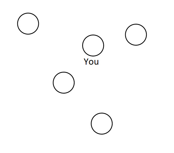
Graphs are made up of 2 things: nodes and edges. Let’s start with nodes. Nodes are the building blocks of a graph. For this example, we’re going to say every node represents a person, including you. Let’s have some collection of nodes, that is a group of people.

Collection of unconnected nodes

In this case, the nodes are not connected at all. It’s just a group of people. Now, since you’re reading this, I know you have friends [I’m one of them :)]. Edges in a graph are used to connect nodes. Let’s add our first edges, shall we? In this case, an edge between 2 people means that these 2 people are friends.

Great! Now, your friends also know other people. So let’s add more edge to complete all the connections between people that we know.

Our fully connected graph!

There! Now you can see through this analogy what a graph actually is. To summarise,

• Graphs are made of nodes and edges

• Nodes make up the graph. Edges connect nodes

• Nodes and edges can represent things and connections in real life

Other common examples of applications of graphs include representing roads connecting cities, connections on social media, the flow of water in pipes, and so on.

Graph terminology

Now that we know what a graph is, let’s learn some of the terminology associated with it. This part is very simple, most of the terminology is exactly what it sounds like.

• A subgraph is a part of a graph

• A connected component is a group of nodes so that I can reach any node from any other node by traversing edges.

  

• A directed graph has edges with directions. Edges can be directed, or bi-directional (un-directed)

  

• A cyclic graph has cycles. An acyclic graph has no cycles. A cycle is when there is a series of directed edges that start and end at the same node

  

• A weighted graph is a graph where edges have values associated with them, called weights. A weight can represent, for example, the length of a road (edge) connecting to cities (nodes).

  

That’s about it. There are some special kinds of graphs, we’ll cover them in a future article. For now, these kinds will be all.

Representing a graph

Remember, in order to represent a graph we need to track 2 things: nodes and edges. There are 3 ways we can represent a graph. Let’s start of with this graph here, and see how it would be represented.

A weighted, directed graph.

Above, we have a weighted, directed graph with nodes 0,1,2,3, and edge weights 1,3,2,-1.

Method 1: Adjacency List

This is the most common way to represent a graph. We call our adjacency list AL.

AL[a] = [(b1,w1), (b2,w2), ...]

AL[a] stores the nodes that node a is connected to. Each pair (b,w) is a directed edge from node a to node b of weight w.

Let’s construct the adjacency list for our graph. Start with node 0. Notice that it’s connected to nothing, so let’s move on.

AL[0] = []

Node 1 is the start of 2 edges. One edge goes from node 1 to 0 of weight 1. Another edge connects it to node 3, with weight -1. Let’s add in that information.

AL[1] = [(0,1), (3,-1)]

Let’s do the same for node 2. It’s connected by edges to nodes 1 and 3.

AL[2] = [(1,3), (3,2)]

Can you see the pattern? Do the same for node 3 now.

AL[3] = [(2,2)]

Our final adjacency list looks like this.

AL = [
[],
[(0,1), (3,-1)],
[(1,3), (3,2)],
[(2,2)],
]

Method 2: Adjacency matrix

This is a matrix, AM.

AM[a][b] = w

In this case, AM[a][b] is a number signifying the weight of an edge connecting node a to node b. It’s simpler than the adjacency list, but takes up a lot more space. If there is no edge between 2 nodes, we can use a placeholder like infinity. In practice, infinity is some pre-defined large constant.

To construct our matrix, simply add in the values for edges that exist.

Method 3: Edge list

This final method is the least commonly used. There are very few reasons to use this, though in certain algorithms it comes in handy.

Exactly what it sounds like, an edge list is a list of edges. Each edge is represented by a tuple.

EL[i] = (a,b,w)

Meaning there is an edge from node a to node b of weight w. The edges in our graph are as follows.

EL = [
(1,0,1),
(1,3,-1),
(2,1,3),
(2,3,2),
(3,2,2)
]

Simple!

Implicit graph

This is a very unique kind of graph. In an implicit graph, we don’t need to store node and edge information because we already know all of it beforehand. This usually relies on special properties of a graph. For example, if every node is connected to every other node by a bi-directional unweighted edge.

Possible implicit graph

We don’t need to store any information for the above graph, because we already know all the vertices and edges. Other examples include grids.

The shortest path problem

One of the most common applications of graphs involves representing some kind of pathway. In this case, we are interested to know, what is the shortest possible path between any 2 nodes in a graph?

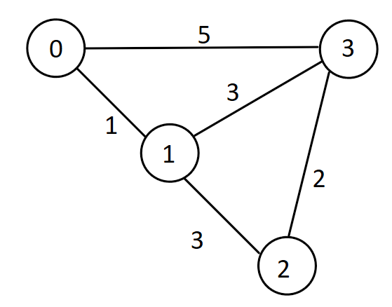
Here’s an example. Suppose every node represents a city, and the cities are connected by bi-directional roads (edges). The weight of each edge represents the length of the road.

Let’s start simple. Say we’re interested in the shortest path from city 0 to every other city. For example, the shortest path from city 0 to 3 has length 3, while that from city 0 to 2 has length 4. How do we solve this problem?

A very clever man with a very fun-to-pronounce name thought about this a long time ago, and came up with a nice solution to the problem.

Edsger W Dijkstra was a very clever man. Image Source: Wikipedia

This man’s name is Edsger W Dijkstra (It’s pronounced Dyke-stra). He invented an algorithm that solves this problem. Let’s see how it works, shall we?

First, we create an array called dist.

int dist[N]; // there are N nodes in the graph
// dist[b] = shortest distance from node 0 to b 

Next, set all values of dist[i] = infinity. Again, in practice, infinity is just a very large constant to signify we can’t reach i from 0 just yet. dist[0] = 0, as the shortest distance from node 0 to itself is obviously 0.

Okay, now consider all direct neighbours of node 0. Realise that we have the shortest distances to each of these nodes, right? So we’re going to do something called “relaxing”. Basically, whenever we relax a neighbour, n, that is a distance d away from 0, we do the following.

dist[n] = d;
pq.insert({d,n}); // pq is a priority queue

pq here is a priority queue we’ve created to store this information. Recall that a priority queue is a queue that is always sorted. In this case, we sort the queue in increasing order of distance.

For every node in the priority queue, we relax all its neighbours. Basically, we’re trying to find better paths as we go along. By the time we’re done, the priority queue is empty.

while (!pq.empty()) { // while pq is not empty
  num d = pq.front().first, n = pq.front().second;
  pq.pop()
  if (d > dist[n]) continue; 
  for (nb : AL[n]) { // for every neighbour of current node
    // get neighbouring node and weight
    node = nb.first, weight = nb.second; 
    if (dist[node] > d + weight) { // if there's a better path
      dist[node] = d + weight; // add the better path
      pq.insert({weight, node});
    }
  }
}

Let’s explore this in practice with our graph.

First, start with node 0.

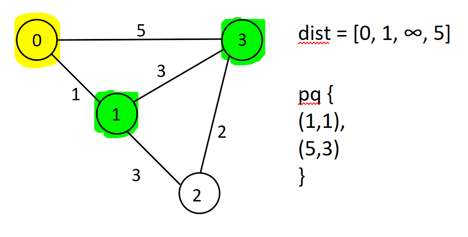
Now, relax all neighbours of 0.

The top of the priority queue is node 1. Let’s consider it. If we do, we’ll find a shorter path to reach node 3- the path from 0 to 1 and then to 3 is shorter than the direct path from 0 to 3. This gets updated.

Great! The process is repeated with node 2, but no shorter path is found. Eventually, all items in the priority queue are removed and our answer is the final answer.

Notice that node 3 appears twice? Well, that’s no problem, since this statement will prevent it from being processed multiple times. Remember we added this line to the code?

if (d > dist[node]) continue; 

It sees the pair (5,3). dist[3] = 4, 5 > 4. So this pair is not processed.

And that’s it! We have our shortest paths all found out! We can repeat this process by changing the starting node to find the shortest paths between any 2 nodes!

Conclusion and future work

Congrats, we’ve successfully learnt what a graph is! In future articles, we’re going to discuss this even further. Graph theory is a beautiful field, too large for a single article.

Some questions we’ll discuss in the future are traversing graphs, colouring graphs, and special graphs called trees. There’s no shortage of topics to cover, but in the meantime, I hope you enjoyed reading this as much as I did writing it. Please like this article if you liked it, the encouragement keeps me going! Thanks for reading, and I’ll see you in the next one!

---

If you enjoy stimulating content like this, subscribe to Elucidate: for the curious coder.

And consider sharing this post if it made your day :)